Research Interests

My main research interests are in physical and bio-medical fluid mechanics and acoustics. This includes numerical modelling involving the development and application of the lattice Boltzmann model. I have also worked with optical measuring techniques such as particle image velocimetry (PIV) and laser induced fluorescence (LIF), again applied to study a variety of interesting fluid phenomenon. Further details of these and other interests can be found below.

The Lattice Boltzmann Model

Transition to Turbulence in Oscillatory Flow

Arterial Simulations

Dispersion of Surface Films

Pulse Reflectometry

Silo Honking

The Lattice Boltzmann Model

The lattice Boltzmann model is a novel technique for simulating fluid motion. The fluid motion is described in terms of the temporal and spatial evolution of the distribution functions f_i, where i  labels the directions on a regular grid. Figure 1 shows a grid which is commonly applied in lattice Boltzmann simulations: the square grid with diagonal. Here the link directions are labeled i =1, 2, ..., 8 and i = 0 corresponds to the rest distribution function.

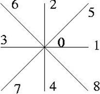
Figure 1: A square grid.

The local fluid density, ρ, and velocity, u, are then calculated at every site, x, and every time-step, t, as

where e_i is the displacement between two sites along link i,  c is the speed with which the distribution functions propagate ( = 1, this term is often dropped in the literature) and b is the number of link directions; here b = 8. The distribution functions evolve according to the lattice Boltzmann equation:

The left-hand-side of equation (1) represents streaming of the distribution functions on the grid. The right-hand-side of equation (1) represents the collisions which occur between the distribution functions. In the lattice Boltzmann model these are usually described by the Bhatnagar, Gross and Krook (BGK) collision function:

where τ is the relaxation time and f_i^eq is the equilibrium distribution function which can be found from the local density and velocity. For the two dimensional square grid shown in figure 1, the equilibrium distribution function is given by

where w₀ = 4/9, w₁=w₂=w₃=w₄=1/9 and w₅=w₆=w₇=w₈ = 1/36.

I am interested in the Lattice Boltzmann Model and its applications. Look at my thesis for further details. 

Return to top of page

Transition to Turbulence in Oscillatory Flow

This work involved an investigation of the transition to turbulence in oscillatory pipe flow.  As well as theoretical interest, oscillatory and pulsating flows have a range of practical applications including oceanography,  oscillatory chemical mixers as well as respiratory and cardiovascular flows.

Oscillatory flows with angular frequency w can be described by two dimensionless numbers: the Reynolds number and the Womersley number. In such flows the Reynolds number is commonly based on the boundary layer thickness: Re_d = U₀d/n, where U₀ is the maximum velocity, n is the kinematic viscosity and d is the boundary layer thickness (d = (2n/w)^1/2). The Womersley parameter is defined by a = a(w/n)^1/2, where a is the pipe radius. A transition to intermittently turbulence flow occurs at Re_d  ~ 500. 

The transition to this intermittently turbulent region does not appear to depend on the Womersley parameter. However, before considering the intermittent turbulence it is interesting to consider the role of the Womersley number. For a <~1 the velocity profile is approximately parabolic and oscillated in phase with the driving force. For large values a >~10 the flow has an 'acoustic' form with an approximately constant velocity across the majority of the pipe, dropping to zero at the walls. Here the velocity is 90^o out of phase with the driving force. At intermediate values the  profile takes on a more interesting shape with a number of points of inflection. These are of interest since at a point of inflection the viscous dissipation term in the Navier-Stokes equation (∇ ²u) is zero. Therefore such points have been linked theoretically to the transition and movement of turbulence in oscillatory flow. Figure 2 shows the profile for four different values of a.

Figure 2: Velocity profile in a pipe of radius a for a range of the Womersley parameter.

A numerical investigation of the transition explained the difference between theoretical and experimental observations concerning the phase of oscillation where the turbulence bursts occurs and identified two instability mechanisms. The primary instability occurs close to flow reversal where a small burst of turbulence occurs in the boundary layer close to the wall. Part of this turbulence is transmitted into the body of the flow along a line of inflection points in the velocity profile. The turbulence which remains in the boundary layer is stretched an twisted by the oscillating fluid before a secondary, much larger, burst of turbulence occurs close to the phase of maximum velocity. Is it the secondary burst of turbulence which is normally observed experimentally and is produced by a Pierrehumbert transition.

For more details of oscillatory flows and the transition to turbulence see the following publications

J. A. Cosgrove, J. M. Buick, S. J. Tonge, C. G. Munro, C. A. Greated and D. M. Campbell. "Application of the lattice Boltzmann method to transition in oscillatory channel flow" Journal of Physics A: Mathematical and General 36: 2609-2620, 2003. [PDF, Journal Link] 

J. A. Cosgrove, J. M. Buick and S. J. Tonge "Evolution of turbulence in an oscillatory flow in a smooth-walled channel: A viscous secondary instability mechanism. Physical Review E 68 Art. No. 026302, 2003. [ PDF Copyright 2003 by The American Physical Society, Journal Link]

Return to top of page

Arterial Simulations

Details coming soon

Return to top of page

Dispersion of Surface Films

The following animation (courtesy of Ted Schlicke) shows the dispersion of a thin surface film due to wave breaking. The images were obtained using laser induced fluorescence. A fluorescent dye was added to the water surface to form a thin film and the system was illuminated with a two-dimensional laser sheet perpendiculars to the water surface. After wave breaking the dispersion of the surface film in the vertical direction and in the direction of wave motion can be observed. The images have been false coloured cording to the concentration of the fluorescent dye. 

Animation 1 (0.6MB)

Animation 2 (6.8MB)

Pulse Reflectometry

I am interested in the development and application of acoustic pulse reflectometry. This is used to measure the internal bore of a cylindrical tube or pipe. An acoustical pulse, generated on a PC, is produced by a speaker at one end of the tube being measured. Inside the tube the pulse is partially reflected every time there is a change in the cross-sectional area. These reflections are recorded by a microphone which is attached to the PC. The reflected signal is then used to reconstruct the internal shape of the pipe. Further details of the technique can be found in David Sharp's thesis html or pdf.

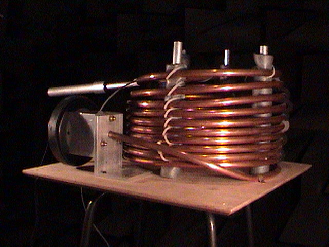
Figure 3. The portable reflectometer. The speaker which produces the sound pulse can be seen on the central left hand side of the picture. This is couple to the copper tube by the aluminium block. Above the speaker a stepped-tube test object can be seen attached to the other end of the copper tube.

Figure 4. Reconstructions of a number of trumpet leadpipes manufactured by Smith-Watkins Brass.

Silo Honking

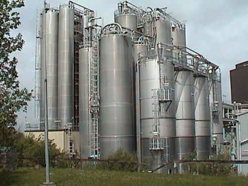
Silo honking occurs in many metal walled silos throughout the world. While the silo is discharging the walls can vibrate with a frequency of a few hundred Hertz and the silo emits a loud `honk'. The honk sounds like a lorry horn and I have measured honks in the 100-110 dB range. The honking phenomenon was investigated on a full scale silo. The bank of silos can be seen in the picture below.
 

 

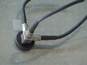
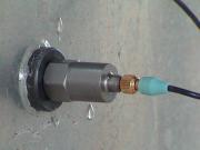
Tri-axial accelerometer, Single accelerometer and Laser Vibrometer