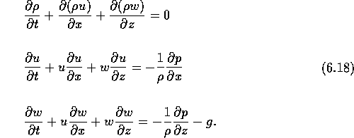
The equations in the preceding section describe interfacial waves at a sharp
interface between two immiscible fluids. The density has a discontinuity at the
interface taking a value ![]() at
at ![]() and
and ![]() at
at ![]() . In
many situations this model may have some shortcomings since there will normally
be a small, but finite, region around the interface where the density changes
smoothly from
. In
many situations this model may have some shortcomings since there will normally
be a small, but finite, region around the interface where the density changes
smoothly from ![]() to
to ![]() . To investigate this phenomenon we will
look at the theory for internal waves in a fluid with a continuously varying
density and then find the solutions for our desired density distribution.
Following references [69, 71] the Sturm-Liouville equation will
be derived which can then be solved numerically for the required density
distribution.
. To investigate this phenomenon we will
look at the theory for internal waves in a fluid with a continuously varying
density and then find the solutions for our desired density distribution.
Following references [69, 71] the Sturm-Liouville equation will
be derived which can then be solved numerically for the required density
distribution.
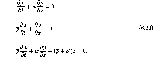
Here we assume, as in the two-fluid case, that the fluid is incompressible,
irrotational and homogeneous. We also make the Boussinesq approximation.
This assumes that density variations are small and can be neglected in so far
as they affect inertia, but retained in the buoyancy terms where they appear
in combination with gravity. The density is given by ![]() where
where ![]() is the mean density and
is the mean density and
![]() is the density fluctuation due to waves motion.
Now the continuity and Navier-Stokes equations are
is the density fluctuation due to waves motion.
Now the continuity and Navier-Stokes equations are
Since the fluid is assumed to be incompressible we can also write
Substituting ![]() into equation (6.18)
and assuming, as before, that the velocities are small and that
into equation (6.18)
and assuming, as before, that the velocities are small and that ![]() is
also small so we can neglect second-order terms in
is
also small so we can neglect second-order terms in ![]() , u, w and
their derivatives, we get
, u, w and
their derivatives, we get
Differentiating the second of these equations with respect to z and the
third with respect to x and noting that ![]() we get
we get
Equating the two terms for ![]() and
differentiating with respect to t and x yields
and
differentiating with respect to t and x yields
Finally we can apply the Boussinesq approximation and set the
right hand side of equation (6.22) to zero since variations in the
density are only important when they occur in combination with gravity.
Now from equations (6.20) and (6.19) we have
![]() and
and
![]() .
Thus equation (6.22) can be re-written in terms of the mean density
.
Thus equation (6.22) can be re-written in terms of the mean density
![]() and the z-component of velocity w as
and the z-component of velocity w as
We look for solutions of equation (6.23) of the form
![]()
which when substituted into equation (6.23) gives
where ![]() where
where
![]() is the
wave celerity and
is the
wave celerity and ![]() where N(z) is the Brunt-Väisälä frequency,
where N(z) is the Brunt-Väisälä frequency,
![]()
Equation (6.25) is the Sturm-Liouville equation and it can not, in
general, be solved analytically. It is however
known [72] that, provided
P(z) > 0, ![]() and R(z) > 0, the Sturm-Liouville equation has
an infinite number of real, positive eigen-value solutions
and R(z) > 0, the Sturm-Liouville equation has
an infinite number of real, positive eigen-value solutions
![]() each with eigen-functions
each with eigen-functions ![]() Each of the eigen-functions
Each of the eigen-functions ![]() having n+1 extremes in the
z-range in which
having n+1 extremes in the
z-range in which ![]() is defined.
For each mode (n=0, 1, ...) there is a unique
relationship between the celerity,
is defined.
For each mode (n=0, 1, ...) there is a unique
relationship between the celerity, ![]() and the wave
number k, this
relationship is referred to as the dispersion relation of that mode.
If we now write the x-velocity in the same form
and the wave
number k, this
relationship is referred to as the dispersion relation of that mode.
If we now write the x-velocity in the same form
![]()
then, from the incompressibility equation (6.19), we find
![]()
If we define
then
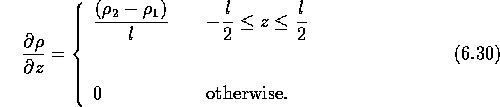
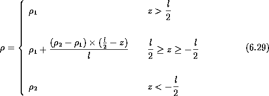
This density distribution is similar to that of the two-layer model except
now the interface is no longer sharp but has a finite size l. The density
changes linearly from ![]() to
to ![]() across the interface.
The lowest mode (n=0) gives a similar motion to the two-layer model while the
higher modes give perturbations to the motion within the interfacial region
l.
To demon straight the difference between the two models the
Sturm-Liouville equation was solved [73] for
across the interface.
The lowest mode (n=0) gives a similar motion to the two-layer model while the
higher modes give perturbations to the motion within the interfacial region
l.
To demon straight the difference between the two models the
Sturm-Liouville equation was solved [73] for ![]() ,
,
![]() , g=0.00015,
, g=0.00015, ![]() ,
,
![]() and l = 5. These are of a similar order to the
values used later
in the lattice Boltzmann simulations. The velocities and wave frequency were
also calculated from equations (6.15) - (6.17) for the
two-layer model. The
z-velocity was found to be virtually the same at all depths for the two
models. The x-velocity was also almost identical except in the interface
region.
The difference between the velocities predicted by the two models is shown
in figure 6-1.
and l = 5. These are of a similar order to the
values used later
in the lattice Boltzmann simulations. The velocities and wave frequency were
also calculated from equations (6.15) - (6.17) for the
two-layer model. The
z-velocity was found to be virtually the same at all depths for the two
models. The x-velocity was also almost identical except in the interface
region.
The difference between the velocities predicted by the two models is shown
in figure 6-1.
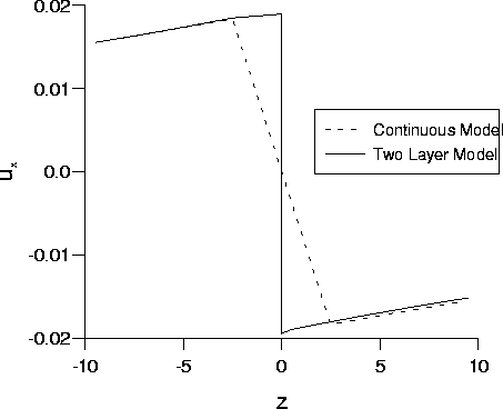
Figure 6-1: The x-velocity predicted by the
two-layer model and the continuous model in the region of the interface.
The values of the frequency ![]() ,
calculated for the two-layer model and the
continuous model were
,
calculated for the two-layer model and the
continuous model were ![]() and
and ![]() respectively,
a difference of about 2.5%.
respectively,
a difference of about 2.5%.