A world was initialised on a 64 by 64 grid with zero velocity and ![]() .
A boundary was placed at the
bottom (z=0) of the grid, which also acted as a boundary at the top,
continuous boundary conditions were applied at the other two edges. Gravity
was then applied using method (1) and method (2) and the density measured
every 1,000 time-steps along a vertical line through the middle of the grid.
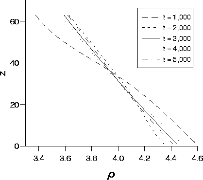
The results are shown in figure 5-1
.
A boundary was placed at the
bottom (z=0) of the grid, which also acted as a boundary at the top,
continuous boundary conditions were applied at the other two edges. Gravity
was then applied using method (1) and method (2) and the density measured
every 1,000 time-steps along a vertical line through the middle of the grid.
The results are shown in figure 5-1

Figure 5-1: Density as a function of
height at selected times
when gravity is applied using method (2).
at times 1,000, 2,000, 3,000, 4,000,
and 5,000 time-steps when gravity is applied
using method (2). The density profile is seen to `oscillate' about its final
position for several thousand time-steps before reaching its final state.
It is clear from figure 5-1 that during this time the distribution
is not symmetric about the mid-height. After 10,000 time-steps the density
at each point is within 0.07% of its final value, at this time the density
distribution is found to lie on the same distribution as that
for t = 3,000 time-steps in figure 5-1 and so is not included
for clarity.
The two methods, method (1) and method (2), were compared by looking at the
difference in the density, ![]() ,
at different heights above the boundary. Here
,
at different heights above the boundary. Here ![]() and
and ![]() are the density when method (1) and method (2)
are used respectively. The results
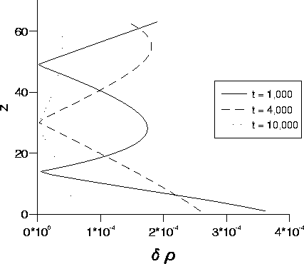
are shown in figure 5-2
are the density when method (1) and method (2)
are used respectively. The results
are shown in figure 5-2

Figure 5-2: The difference in density between method (1) and
method (2) as a function of height at selected times.
at times 1,000 4,000 and 10,000 time-steps. The size of the density difference
is small compared to the mean density of 4 and is seen to decrease with time.
After 1,000 time-steps it has a maximum value of ![]() ,
only 0.025% of the mean density, at subsequent times the difference is
always smaller. The shape of the graphs shown in figure 5-2 are
typical of the shape of all the results obtained.
Consider either method applied to an infinite fluid with the same initial
density at each site. There is no density change induced at any of the sites
by the gravitational force. On our finite grid a
small difference will occur at
sites adjacent to the boundary and these will propagate through the fluid.
The difference in the update rules at these sites
account for the small variations observed here,
which are negligibly small, and for the shape of the curves in
figure 5-2. Thus both method (1) and method (2)
are producing the same effect. This is to be expected since they both
satisfy the same equations of motion.
,
only 0.025% of the mean density, at subsequent times the difference is
always smaller. The shape of the graphs shown in figure 5-2 are
typical of the shape of all the results obtained.
Consider either method applied to an infinite fluid with the same initial
density at each site. There is no density change induced at any of the sites
by the gravitational force. On our finite grid a
small difference will occur at
sites adjacent to the boundary and these will propagate through the fluid.
The difference in the update rules at these sites
account for the small variations observed here,
which are negligibly small, and for the shape of the curves in
figure 5-2. Thus both method (1) and method (2)
are producing the same effect. This is to be expected since they both
satisfy the same equations of motion.